Learning & methods · November 2026学习与方法 · 2026 年 11 月
When Better Preference Fitting Makes a Worse Policy偏好拟合得更好,为什么策略反而变差?
A three-action example reveals how a restricted policy family and pair frequencies can misdirect DPO—and why AuxDPO separates policy movement from preference fitting.从一个三动作算例理解 DPO 的模型错配:策略能表达什么、哪些比较出现得更多,以及 AuxDPO 怎样把两种自由度分开。
The equivalence starts with an unrestricted policyDPO 的等价关系,先从自由策略出发
偏好数据更丰富,优化器也把损失降得更低,模型为什么仍可能更差?关键不一定是标签噪声,而可能是模型类错配:真实偏好的概率结构不在模型能够表达的范围里,拟合只能作出折中。AuxDPO 论文讨论的是这个具体条件,不是证明“DPO 从一开始就是错的”。
固定问题 x,设参考策略为 ,真实奖励为 。在参考支持集上,若允许自由选择任意响应分布,最大化 的解是:
反解奖励,再将其代入 Bradley–Terry 偏好概率,问题内共同的 会在分数差中消失。于是可以用策略的相对对数概率构造“隐式奖励”:
这就是 DPO 将偏好拟合直接写成策略参数损失的入口。困难在下一步:神经网络参数共享、冻结层或有限适配器,并不允许每个响应概率独立调整。所有 形成一个受约束集合;真实奖励在扣除问题内无关常数后,也可能不在其中。此时“自由分布的闭式解”不能直接当作受限模型类中训练结果的保证。DPO 原论文 §4 与附录 A给出前述变量变换;AuxDPO §2–3研究受限策略类中的差异。
Why can more preference data and a lower optimized loss still produce a worse policy? Label noise is not the only explanation. Under model misspecification, the probability structure of true preferences lies outside the model's representational family, so fitting requires compromises. The AuxDPO paper studies this condition; it does not establish that DPO is universally wrong.
For a fixed prompt x, let the reference be and true reward be . If any response distribution on the reference support is allowed, maximizing gives:
Invert this relation and substitute the reward into Bradley–Terry preference probabilities. The prompt-specific constant cancels in a reward difference, giving an implicit reward from relative policy log probabilities:
This lets DPO express preference fitting directly in policy parameters. The difficulty comes next: shared network parameters, frozen layers, or restricted adapters do not permit independent adjustments of every response probability. The family of is constrained. Even after allowing an irrelevant prompt-specific constant, the true reward may lie outside it. An optimum over free distributions is then not automatically a guarantee for training within the restricted family. DPO §4 and Appendix A derive the transformation; AuxDPO §2–3 examine the restricted-policy setting.
Pair frequencies determine the compromise比较出现得多,就在折中中更有分量
令 为真实偏好概率, 为模型预测。若比较 i、j 的频率是 ,无限数据下的期望 DPO 损失仍是加权二元交叉熵:
利用 ,其中 H(q) 不随参数变化,训练等价于寻找一组可表达的偏好概率,使这个带比较频率权重的误差最小。这里明确写出 KL 的两个参数;它是偏好 Bernoulli 分布之间的 KL,不是策略与参考策略之间的 KL。
如果所有偏好都能准确表达,各项误差可以同时降为零;如果不能,增加某种比较的权重就会改变折中。更多数据可以更准确地确定这个受约束最优解,却不保证它就是期望奖励最大的策略。要区分两件事:有限样本造成的估计误差,以及即使无限数据也存在的表达限制。后者是本文主问题。上述分解对应 AuxDPO 命题 1,交叉熵本身的推导可接着阅读本站的 Bradley–Terry 图解。
Let denote true preference probabilities and the model's predictions. If the comparison frequency for i and j is , the population DPO loss remains a weighted binary cross-entropy even with unlimited data:
Use . Because H(q) does not depend on parameters, training seeks expressible preference probabilities minimizing this error weighted by comparison frequencies. The arguments are explicit: this KL is between Bernoulli preference distributions, not between the policy and its reference.
If all preferences are realizable, every term can be minimized simultaneously. If not, increasing one type of comparison changes the compromise. More data can identify that constrained optimum more precisely without making it the policy that maximizes expected reward. Separate finite-sample estimation error from representational restrictions that remain with unlimited data. The latter is our focus. This decomposition is AuxDPO Proposition 1; the site's Bradley–Terry explainer develops the cross-entropy connection.
Three actions make the conflict concrete三个动作,就能把矛盾算出来
沿用论文命题 3 的结构,固定一个问题,三个动作的奖励为 。最好的是 a₂,最差的是 a₃。策略却只有一个可调参数:
提高 a₁ 的概率时,a₂ 会被压低;提高 a₂ 时,a₁ 又会落到 a₃ 下方。这个家族根本无法同时表达 a₂ > a₁ > a₃ 的完整排序。基准策略均匀采样,期望奖励恰为 1。
令 。对比较 (1,2)、(2,3)、(3,1),模型偏好 logit 精确地是 ,因为共同的归一化项会消掉;真实 logit 则是 。第二对希望 c 为负,第三对希望 c 为正,两者无法都满足。
Use the structure of Proposition 3: one prompt, three actions, and rewards . Action a₂ is best and a₃ is worst. The policy has only one adjustable parameter:
Increasing a₁ suppresses a₂; increasing a₂ moves a₁ below a₃. This family cannot represent the full ordering a₂ > a₁ > a₃. Its uniform reference policy has expected reward exactly 1.
Write . For comparisons (1,2), (2,3), and (3,1), the model's preference logits are exactly because the common normalization cancels. The true logits are . The second pair wants negative c; the third wants positive c. Both cannot be satisfied.
Static diagram静态图
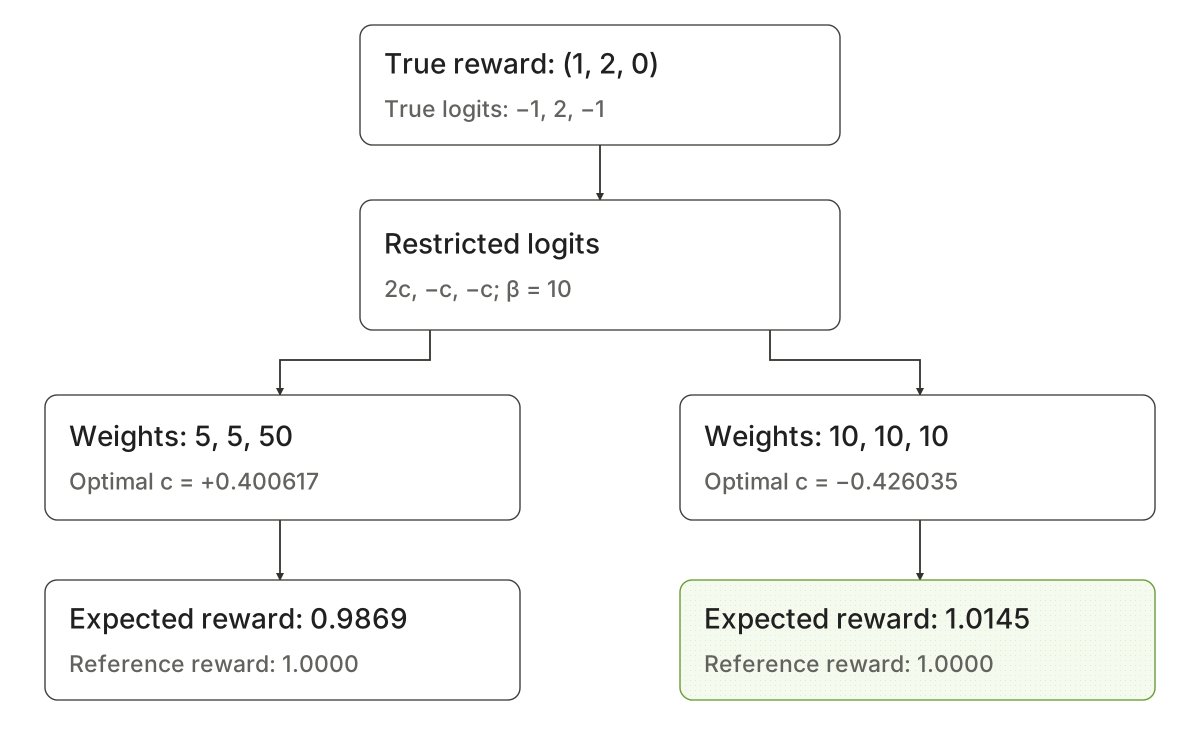
下面是对该结构额外选择权重后,直接求解总体损失的教学计算,不是论文的模型实验。固定 β=10;权重代表比较频率,不是声称抽到这些数量的标签就恰好等于总体概率。
| 比较权重 (12,23,31) | 最优 c | 策略 π(a₁,a₂,a₃) | 期望奖励 |
|---|---|---|---|
| 基准 | 0 | (0.3333, 0.3333, 0.3333) | 1.0000 |
| (5,5,50) | 0.400617 | (0.3468, 0.3201, 0.3332) | 0.9869 |
| (10,10,10) | −0.426035 | (0.3192, 0.3476, 0.3331) | 1.0145 |
不平衡情形的平均交叉熵从 0.693147 降到 0.668933,而奖励从 1 降到 0.986917:优化器确实把自己的损失改善了,却更少选择最优动作。平衡权重在本例中改变方向,并不证明平衡采样可以修复所有模型错配。两行损失也属于不同加权目标,不能直接拿它们互相排名。
The following is an additional teaching computation using chosen comparison weights and directly optimizing the population loss, not an LLM experiment from the paper. Fix β=10. The weights represent comparison frequencies; they do not imply that a finite set of that many labels exactly equals the population probabilities.
| Pair weights (12,23,31) | Optimal c | Policy π(a₁,a₂,a₃) | Expected reward |
|---|---|---|---|
| Reference | 0 | (0.3333, 0.3333, 0.3333) | 1.0000 |
| (5,5,50) | 0.400617 | (0.3468, 0.3201, 0.3332) | 0.9869 |
| (10,10,10) | −0.426035 | (0.3192, 0.3476, 0.3331) | 1.0145 |
In the imbalanced case, mean cross-entropy falls from 0.693147 to 0.668933 while reward drops from 1 to 0.986917. The optimizer genuinely improves its own objective while selecting the best action less often. Balancing the weights changes direction here; it is not a general cure for misspecification. The rows also optimize differently weighted losses, so their loss values should not be ranked against one another.
Policy improvement needs only part of the reward information策略需要的奖励信息,比完整偏好更少
AuxDPO 的思路来自另一侧:奖励的哪些变化会影响策略更新?在参考点附近,令 ,把这些向量排成矩阵 G;令 D 的对角线是参考动作概率,记 、。这里省略固定问题;一般情况还要按问题分布加权。
把期望奖励作一阶展开、策略 KL 作二阶展开,局部目标为:
因此最小范数的局部最优增量为 。符号 † 是伪逆。策略此时依赖的是 ,而非奖励向量的每一维。若 ,把奖励加上 δ 不改变这一局部更新信号。
在三动作例中,、、,故 。奖励可以拆成 :前一项指向提高 a₂ 的局部策略更新;后一项落在 B 的零空间,改变偏好细节,却不改变参考点上的一阶奖励梯度。
AuxDPO approaches the problem from the other side: which changes in reward affect policy improvement? Around the reference, let and collect these vectors as columns of G. Let D contain reference action probabilities on its diagonal, with and . We suppress the fixed prompt; multiple prompts also require prompt-distribution weights.
A first-order expansion of expected reward and a second-order expansion of policy KL give:
The minimum-norm local optimum is therefore , where † denotes the pseudoinverse. The policy depends on , not every reward coordinate separately. If , adding δ does not change this local update signal.
In the three-action example, , , and , so . Decompose the reward as . The first component points toward locally increasing a₂. The second lies in B's null space: it changes preference details without changing the first-order reward gradient at the reference.
Static diagram静态图
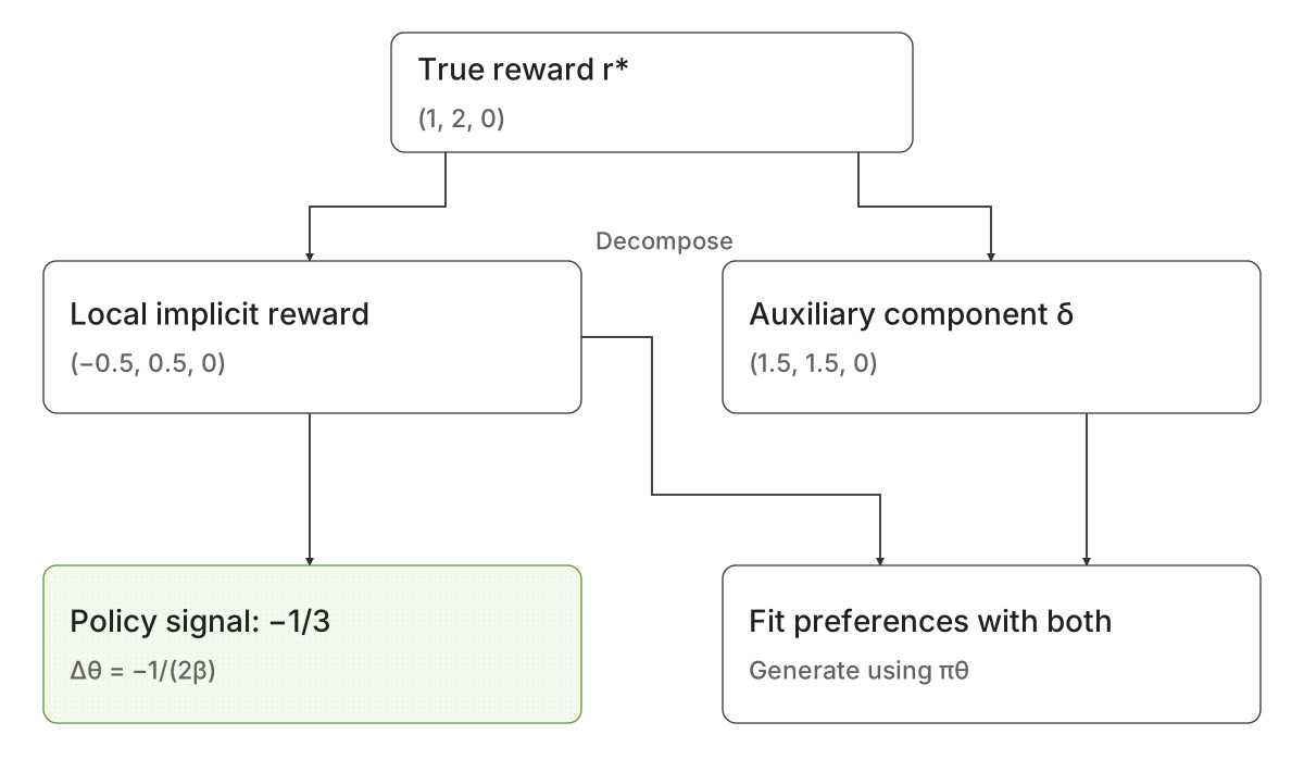
这不是说后一项“永远没用”。它只是在该参考策略与该局部近似下不改变一阶更新;离开参考点后几何会变化。AuxDPO §4.1正是借助这个受限的等价关系,而不是声称所有奖励都可以无损压成一个标量。
The second component is not permanently irrelevant. It preserves the first-order update only at this reference and within this approximation; the geometry changes away from the reference. AuxDPO §4.1 uses this limited equivalence, not a claim that arbitrary rewards can be compressed losslessly into a single number.
Auxiliary variables absorb residuals without enlarging the policy辅助变量吸收偏好残差,不扩张策略家族
普通 DPO 让策略参数同时承担两件事:拟合成对偏好、决定生成行为。AuxDPO 允许隐式奖励外再加一个受约束分量:
偏好损失改用 的分数差。为了看清尺度,这里 δ 采用奖励单位,因此一对样本的 margin 是 ;若实现把辅助量放在 β 括号里,就需相应重定义其单位。重要的不是随便加可调偏置,而是让它受零空间条件约束:如果每对标签都能任意修改 margin,辅助量可能独自记住标签,策略却不改善。
论文的总体分析在局部、大 β 条件下建立联系;有限数据实现则用样本近似和约束或惩罚处理辅助量。大模型上得到一个惩罚较小的解,不等于已经严格满足总体零空间条件。辅助变量也不会让三动作例的一个参数突然表达任意排序:它使拟合偏好的自由度更丰富,生成时的策略仍属于原家族。
就三动作教学例而言,零空间分解解释了为何局部策略应朝负 θ 方向,而不要求恢复完整的 a₂ > a₁ > a₃ 排序。它是机制解释;本文没有运行 AuxDPO 大模型训练,也不把这个分解当作新实验结果。约束与有限样本形式见 论文 §4.2。
Ordinary DPO asks policy parameters to do two jobs: fit pairwise preferences and determine generation behavior. AuxDPO permits a constrained component outside the policy's implicit reward:
The preference loss now uses differences of . To make the scale explicit, δ here has reward units, so a sample's margin is . An implementation placing the auxiliary term inside the β brackets must redefine its units accordingly. The point is not to add arbitrary adjustable biases: the null-space condition matters. If every pair could change its margin freely, auxiliary variables could memorize labels without improving the policy.
The population analysis establishes its connection in a local, large-β regime. Finite-data implementations approximate the relevant quantities and use constraints or penalties. A small penalty in a large-model run is not proof that the exact population null-space condition holds. Auxiliary variables also do not let the one-parameter example express arbitrary action orderings. They enrich preference-fitting freedom while leaving the generating policy in its original family.
For the teaching example, the null-space decomposition explains why the local policy should move toward negative θ without requiring recovery of the complete a₂ > a₁ > a₃ ordering. This is a mechanism explanation. We have not run large-model AuxDPO training and do not present this decomposition as a new empirical result. See §4.2 for the constraints and finite-sample formulation.
Evaluate the generating policy, not only its preference loss评估的是生成策略,不能只看偏好 loss
这个结果改变的是判断训练的方式。比较数据覆盖了哪些答案对、模型允许哪些联合概率变化、优化目标怎样加权这些比较,都能影响最终策略。它们与“标签对不对”是不同维度;数据干净也不自动消除表达限制。
如果要比较 DPO 与 AuxDPO,应在相同底座、数据、可训练参数、训练与生成预算下,分别看偏好拟合、真实生成结果以及跨任务评测。为辅助变量带来的额外优化成本单列记录。不能仅以训练 loss 更低宣布方法更好,也不能把三动作反例推广成“现实中的 DPO 必然失败”。
一个最有用的结论是:拟合得更准,必须先问拟合的是什么,以及模型被允许怎样改变。Bradley–Terry 的交叉熵解释了如何学习偏好;模型错配则说明,偏好预测、奖励表示与生成策略这三层,不能总是无条件地互相替代。
The result changes how we judge training. Which answer pairs are compared, which joint probability changes the model permits, and how the objective weights those comparisons can all affect the final policy. These are separate from label correctness; clean data do not automatically remove representational restrictions.
To compare DPO and AuxDPO, hold the base model, data, trainable policy parameters, training budget, and generation budget comparable, then measure preference fitting, actual generated outcomes, and cross-task evaluation separately. Record the additional optimization cost of auxiliary variables. A lower training loss does not establish a better method, and a three-action counterexample does not establish that DPO inevitably fails in practice.
The useful conclusion is: better fitting only becomes meaningful after identifying what is being fit and how the model is allowed to change. Bradley–Terry cross-entropy explains preference learning. Misspecification shows why preference prediction, reward representation, and the generating policy are not always interchangeable without conditions.
Continue reading继续阅读
- Gopalan, Chowdhury & Banerjee: Why DPO is a Misspecified Estimator and How to Fix It (v1)
- Rafailov et al.: Direct Preference Optimization (v2), §4 and Appendix A
- Original study notes原始学习笔记 · auxdpo explained
- Original study notes原始学习笔记 · auxdpo source